Table of Contents
This interface is used to reduce ISIS SANS data for SANS2D, LOQ,LARMOR and ZOOM. The interface can be accessed from the main menu of MantidPlot, in Interfaces → SANS → ISIS SANS. This interface is intended as a gradual replacement for the old ISIS SANS interface. As of version 4.0 this interface was renamed from ISIS SANS v2 experimental to ISIS SANS, and the previous SANS interface was deprecated. This change signifies that this interface provides all major functionality and will be the only ISIS SANS interface subject to active development.
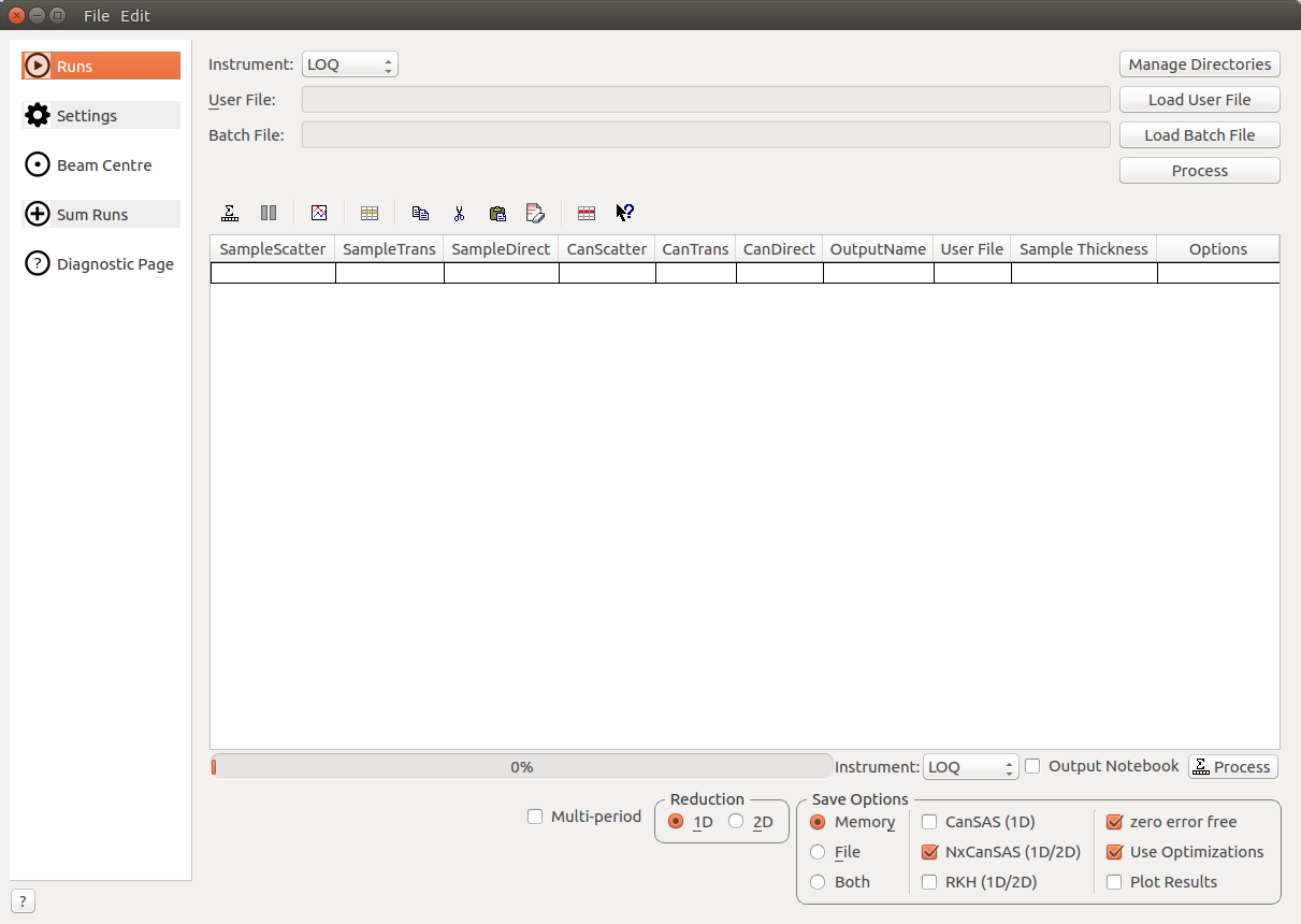
The Runs tab is the ISIS SANS entry-point. It allows the user to specify the user file and batch file. Alternatively the user can set the data sets for reduction manually on the data table. In addition it allows the user to specify her preferred save settings (see more below). The actual parameters which are loaded from the user file are accessible from the sub-tabs on the Settings tab.
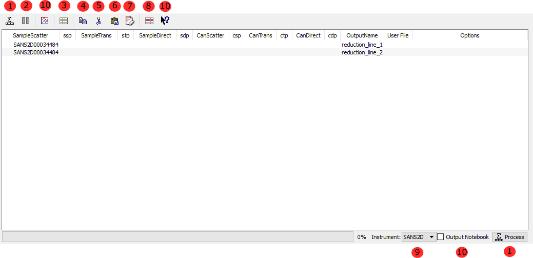
| 1 | Process | If no individual row is selected in the data table, then this will start a reduction. In this case the user will be asked if she is sure that she wants to reduce all rows. If rows are selected, then only these will be processed. |
| 2 | Pause | Allows the user to pause a reduction, change her row selection and continue the reduction with possibly a different selection. |
| 3 | Insert row after | Adds a row after the currently selected row. |
| 4 | Copy selected | Creates a copy of the selected rows. |
| 5 | Cut selected | Cuts the selected rows. |
| 6 | Paste selected | Pastes rows from the clipboard. |
| 7 | Clear selected | Clears the entries from selected rows. It however does not the delete the rows themselves. |
| 8 | Delete row | Deletes a selected row. |
| 9 | Select instrument | Selects the instrument to use. Note that this setting is used to resolve run numbers. |
| 10 | Unused Functionality | These icons are not used |
| SampleScatter | Scatter data file to use. This is the only mandatory field |
| ssp | Sample scatter period, if not specified all periods will be used (where applicable) |
| SampleTrans | Transmission data file to use. |
| stp | Sample scatter period, if not specified all periods will be used (where applicable) |
| SampleDirect | Direct data file to use |
| sdp | Sample direct period, if not specified all periods will be used (where applicable) |
| CanScatter | Scatter datafile for can run |
| csp | Can scatter period, if not specified all periods will be used (where applicable) |
| CanTrans | Transmission datafile for can run |
| ctp | Can transmission period, if not specified all periods will be used (where applicable) |
| CanDirect | Direct datafile for can run |
| OutputName | Name of output workspace |
| User File | User file to use for this row. If specified it will override any options set in the GUI, otherwise the default file will be used. |
| Sample Thickness | Sets the sample thickness to be used in the reduction. |
| Options | This column allows the user to provide row specific settings. Currently only WavelengthMin , WavelengthMax and EventSlices can be set here. |
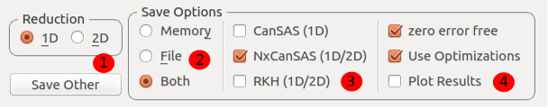
| 1 | Save Other | Opens up the save other dialog box Save Other which allows for manual saving of reduced data. |
| 2 | Save location | This sets where the reduced data will be made available for the user. The user can select to have it only in memory (RAM) with the Memory option, saved out as a file with the File option or saved both to file and memory with the Both option. |
| 3 | Save file formats | Allows the user to specify the save file format for the reduced data. |
| 4 | Other | The zero error free option ensures that zero error entries get artificially inflated when the data is saved to a file. This is beneficial if the data is to be loaded into other analysis software. The Use optimizations option will reuse already loaded data. This can speed up the data reduction considerably. It is recommended to have this option enabled. The Plot results option controls whether the reduced data is automatically plotted to a graph or not. |
The Settings tab and its sub-tabs allow for manipulating and inspecting the reduction parameters which were initially set through loading a user file. Currently there are five sub-tabs:
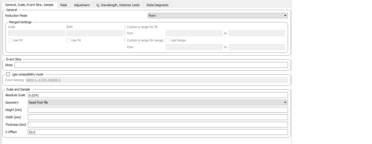
The first tab contains settings which are not associated with the wider themes of the other tabs.
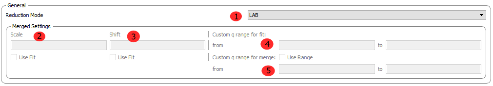
| 1 | Reduction mode | The user can choose to either perform a reduction on the low angle bank (LAB), the high angle bank (HAB), on both (Both) or she can perform a merged (Merged). If a merged reduction is enabled, then further settings are required (see below). A merged reduction essentially means that the reduced result from the low angle bank and the high angle bank are stitched together. |
| 2 | Merge scale | Sets the scale of a merged reduction. If the Fit check-box is enabled, then this scale is being fitted. |
| 3 | Merge shift | Sets the shift of a merged reduction. If the Fit check-box is enabled, then this shift is being fitted. |
| 4 | Merge fit custom q range | Describes the q region which should be used to determine the merge parameters. |
| 5 | Merge custom q range | Describes the q region in which the merged data should be used. Outside of this region the uncombined HAB or LAB data is used. |

In case of data which was measured in event-mode, it is possible to perform time-of-flight slices of the data and reduce these separately. The input can be:
In addition it is possible to concatenate these specifications using comma-separation. An example would be 5-10,12:2:16,20-30.

The old SANS GUI allows event-mode data as input but will convert it early on into histogram-mode data, either using the time-of-flight binning parameters specified by the user or by using the binning inherent to the monitors. The new SANS GUI can handle event-mode data up to the conversion to momentum transfer. This leads to more precise results. However if the user wishes to compare the results between the two GUIs she is advised to enable the compatibility mode. This will ensure that event-mode data will be converted to histogram-mode data early on, even in the new reduction framework and will lead to the same results as one expects from the old GUI.
If the check-box is enabled, then the time-of-flight binning parameters will be taken from the Event binning input. If this is not set, then the binning parameters will be taken from the monitor workspace.
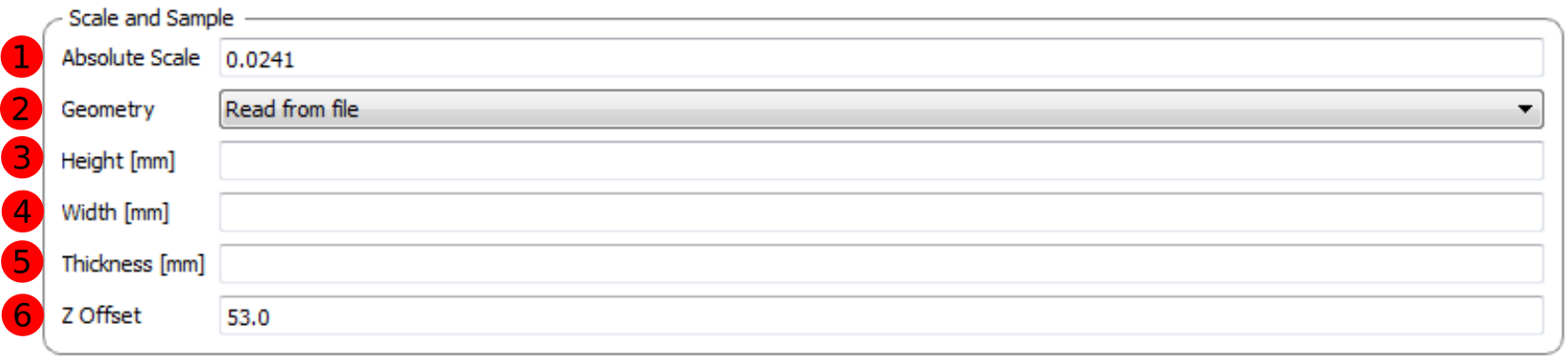
This grouping allows the user to specify the absolute scale and sample geometry information. Note that the geometry information is in millimetres.
| 1 | Absolute scale | The absolute, dimensionless scale factor. |
| 2 | Geometry | A geometry selection. Read from file will use the settings that are stored in the data file. The other options are Cylinder, FlatPlate and Disc. |
| 3 | Height | The sample height. If this is not specified, the information from the file will be used. |
| 4 | Width | The sample width. If this is not specified, the information from the file will be used. |
| 5 | Thickness | The sample thickness. If this is not specified, the information from the file will be used. |
| 6 | Z offset | The sample offset. |
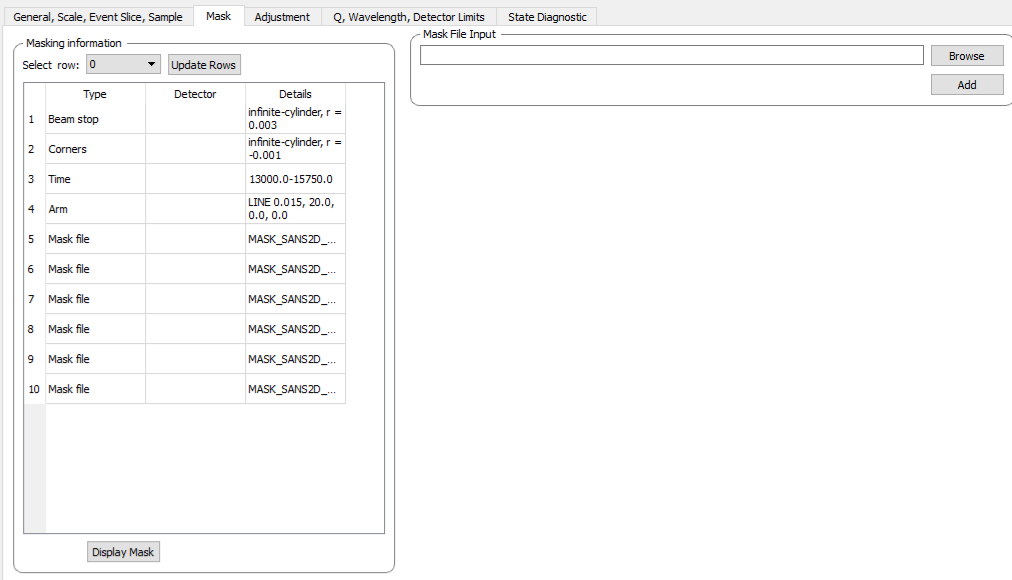
The elements on this tab relate to settings which are used during the masking step.
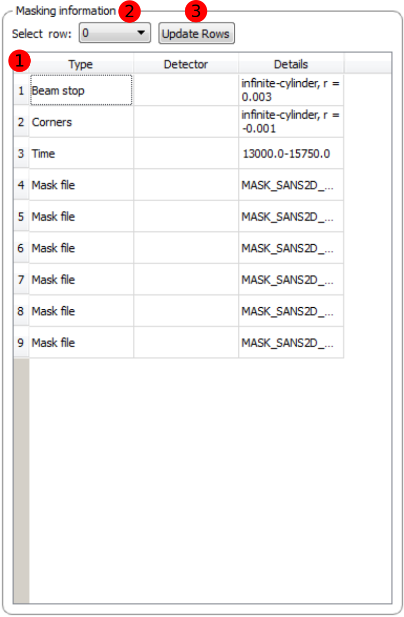
The masking table shows detailed information about the masks which will be applied. These masks include bin masks, cylinder masks, mask files, spectrum masks, angle masks and line masks for the beam stop arm. If a mask is applied only to a particular detector then this will be shown in the masking table. Note that data needs to be specified in order to see the masking information. Also note if a manual change to the data table or other settings, requires you to update the row selection by pressing Update Rows.
| 1 | Table | The masking table which displays all masks which will be applied to the data set. |
| 2 | Select row | The masking information is shown for a particular data set in in the data table. The information for the selected row is shown. |
| 3 | Update rows | Press this button if you have manually updated the data table. These changes are currently not picked up automatically. |
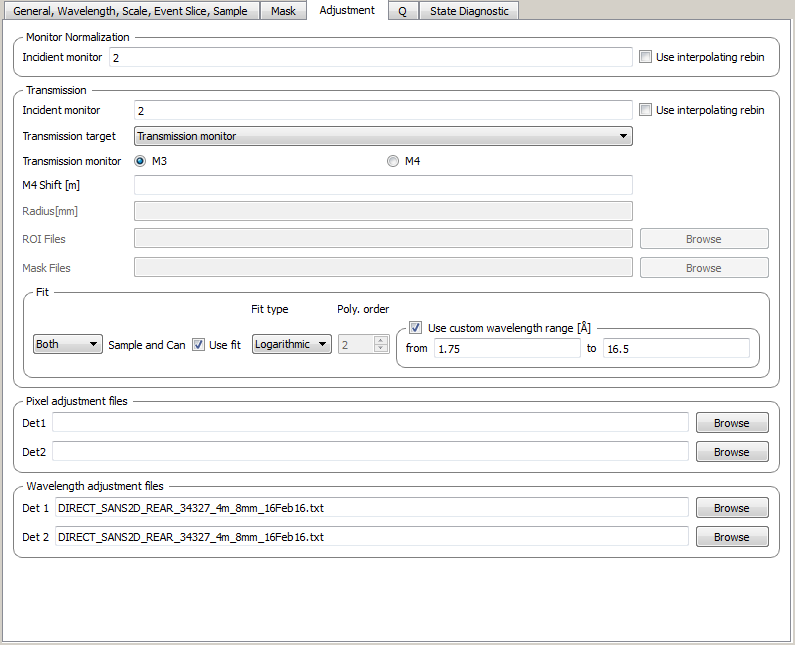
This tab provides settings which are required for the creation of the adjustment workspaces. These adjustments include monitor normalization, transmission calculation and the application of adjustment files.

| 1 | Incident monitor | The incident monitor spectrum number. |
| 2 | Use interpolating rebin | Check if an interpolating rebin should be used instead of a normal rebin. |
The main inputs for the transmission calculation are concerned with the incident monitor, the monitors/detectors which measure the transmission and the fit parameters for the transmission calculation.
| 1 | Incident monitor | The incident monitor spectrum number. |
| 2 | Use interpolating rebin | Check if an interpolating rebin should be used instead of a normal rebin. |
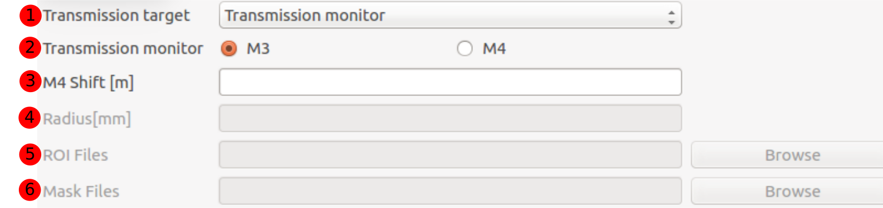
| 1 | Transmission targets | This combo box allows the user to select the transmission target. Transmission monitor will take the transmission data from the monitor which has been selected in the Transmission monitor field. Region of interest on bank will take the transmission data from the fields Radius, ROI files and Mask files. |
| 2 | Transmission monitor | The monitor which will be used for the transmission calculation. |
| 3 | M4 shift | An optional shift for the M4 monitor. |
| 4 | Radius | This will select all detectors in the specified radius around the beam centre to contribute to the transmission data. |
| 5 | ROI files | A comma-separated list of paths to ROI files. The detectors specified in the ROI files contribute to the transmission data. |
| 6 | Mask files | A comma-separated list of paths to Mask files. The detectors specified in the Mask files are excluded from the transmission data. |
Additional information:
As mentioned above the transmission target can be a monitor (e.g. M3 or M4) or a region of interest on the detector bank itself. If the preferred target is a selection of pixels on the detector bank itself, then the user can specify a region of interest. The pixels in the region of interest contribute to the transmission calculation. There are several ways to specify the region of interest:
The combination of both methods can also be specified. This results in the union of all relevant pixels. In order to avoid certain areas on the detector, a list of Mask-files can be specified. The Mask file is equivalent to a mask file created in the Instrument View Window. Note that this mask file is only used for the transmission calculation.
The most general selection on the detector bank will be a specified radius, a list of ROI files and a list of Mask files. Note that individual pixels which are specified by either the radius setting or a ROI file and at the same time by the Mask file, will not be considered for the transmission calculation.
The following example/image should help to clarify the selection process:
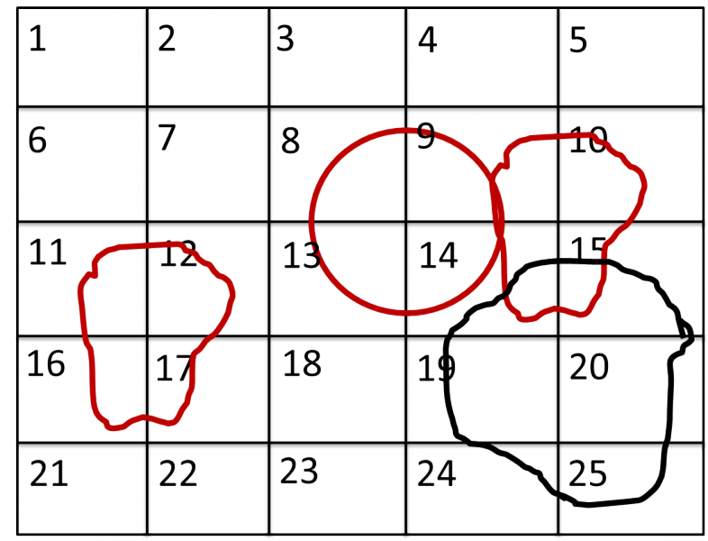
The radius selection (red) picks pixels 8, 9, 13 and14. The ROI files (red) select pixels 9, 10, 11, 12, 14, 15, 16 and 17. This means pixels 8 to 17 are selected. The Mask file (black) selects pixels 14, 15, 19, 20, 24 and 25. This means that pixels 14 and 15 are dropped and pixels 8, 9, 10, 11, 12, 13, 16 and 17 are being used in the final transmission calculation.
| 1 |
|
|||
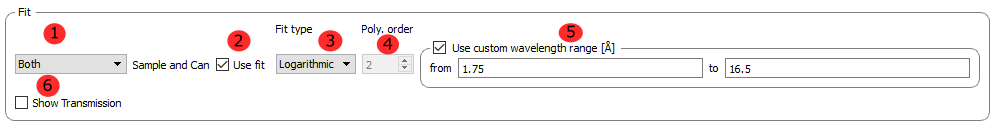
| 2 | Use fit | If fitting should be used for the transmission calculation. | ||
| 3 | Fit type | The type of fitting for the transmission calculation This can be Linear, Logarithmic or Polynomial. | ||
| 4 | Polynomal order | If Polynomial has been chosen in the Fit type input, then the polynomial order of the fit can be set here. | ||
| 5 | Custom wavelength | A custom wavelength range for the fit can be specified here. | ||
| 6 | Show Transmission | Controls whether the transmission workspaces are output during reduction. | ||
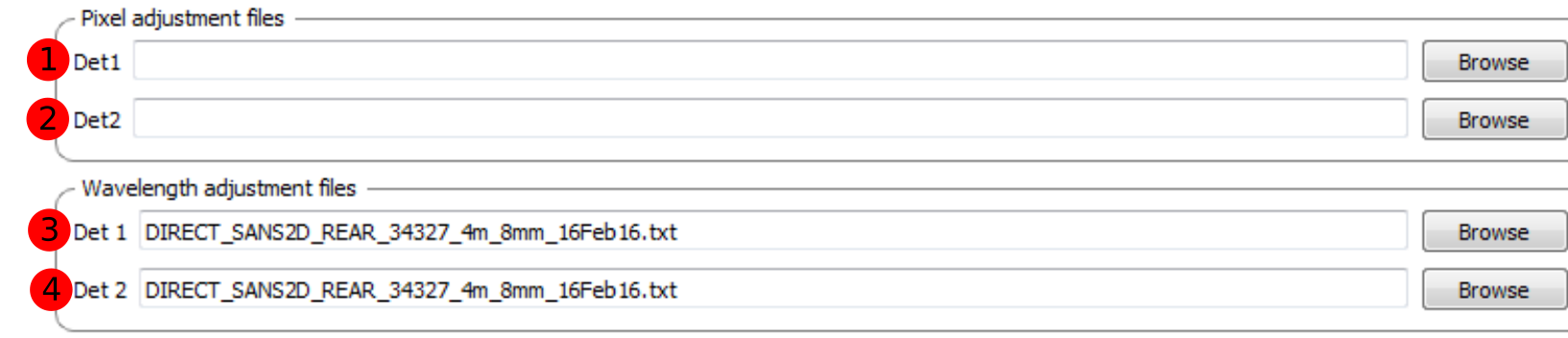
| 1 | Pixel adjustment det 1 | File name of the pixel adjustment file for the first detector. The file to be loaded is a ‘flat cell’ (flood source) calibration file containing the relative efficiency of individual detector pixels. Note that the numbers in this file include solid angle corrections for the sample-detector distance at which the flood field was measured. On SANS2D this flood field data is then rescaled for whatever sample-detector distance the experimental data was collected at. This file must be in the RKH format and the first column a spectrum number. |
| 2 | Pixel adjustment det 2 | File name of the pixel adjustment file for the second detector. See more information above. |
| 3 | Wavelength adjustment det 1 | File name of the wavelength adjustment file for the first detector. The content specifies the detector efficiency ratio vs. wavelength. These files must be in the RKH format. |
| 4 | Wavelength adjustment det 2 | File name of the wavelength adjustment file for the second detector. See more information above. |
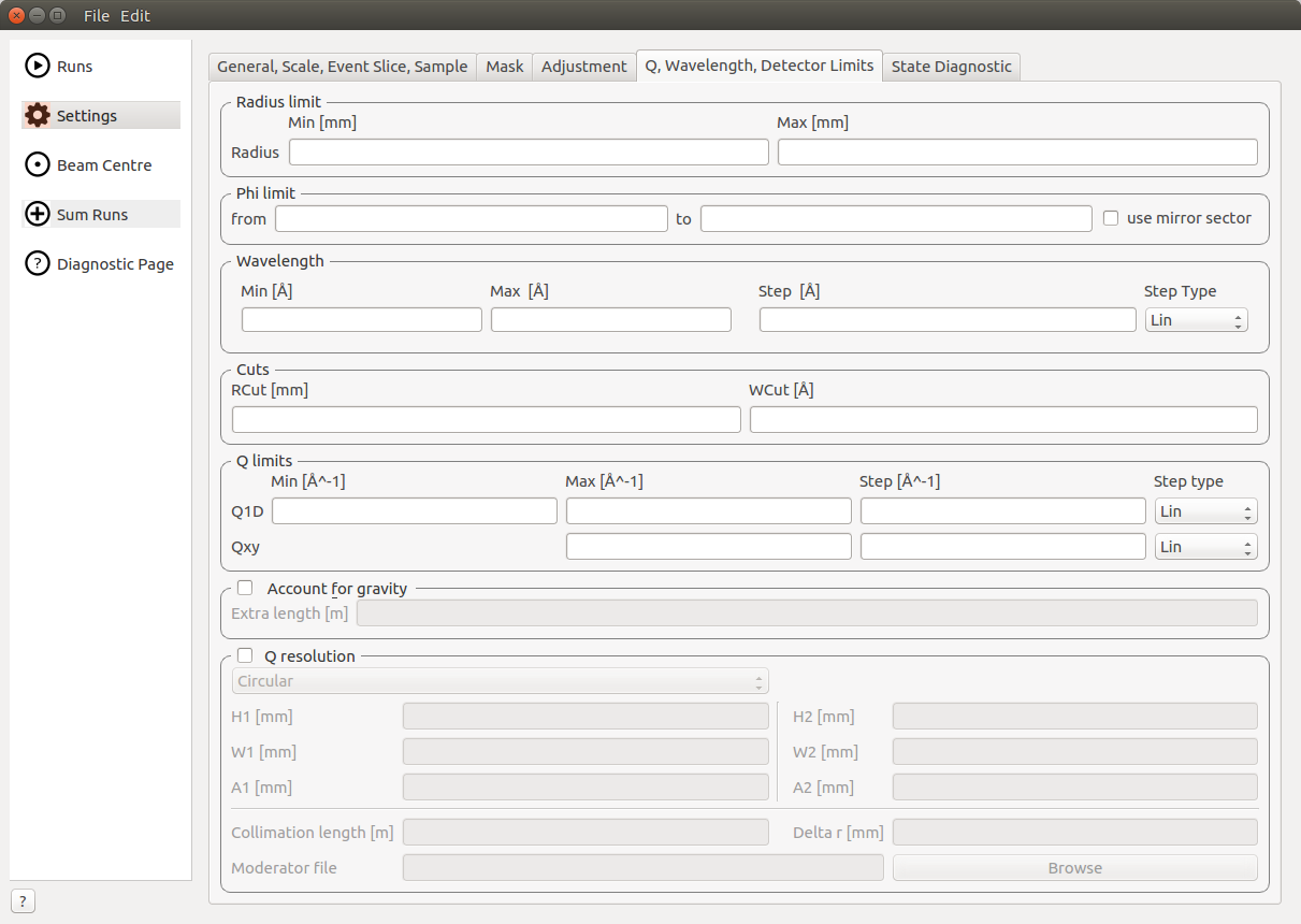
The elements on this tab relate to settings which are used during the conversion to momentum transfer step of the reduction.
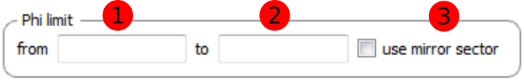
This group allows the user to specify an angle (pizza-slice) mask. The angles are in degree.
| 1 | Start angle | The starting angle. |
| 2 | Stop angle | The stop angle. |
| 3 | Use mirror | If the mirror sector should be used. |
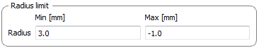
These settings allow for a hollow cylinder mask. The Min entry is the inner radius and the Max entry is the outer radius of the hollow cylinder.

The settings provide the binning for the conversion from time-of-flight units to wavelength units. Note that all units are Angstrom. Depending on which Step type you have chosen you will be asked to enter either a Max and Min wavelength value between which to do the reduction or to specify a set of wavelength ranges to reduce between. The syntax for the latter case is the same as that used to specify event slices and is
In addition it is possible to concatenate these specifications using comma-separation. An example would be 5-10,12:2:16,20-30.
| 1 | Min | The lower bound of the wavelength bins. |
| 2 | Max | The upper bound of the wavelength bins. |
| 3 | Step | The step of the wavelength bins. |
| 4 | Step type | The step type of the wavelength bins, i.e. linear, logarithmic range linear or ranged logarithmic. |
| 5 | Ranges | A set of wavelength ranges. This option only appears if a range step type is selected. |

These allow radius and wavelength cuts to be set. They are passed to Q1D as the RadiusCut and WaveCut respectively.
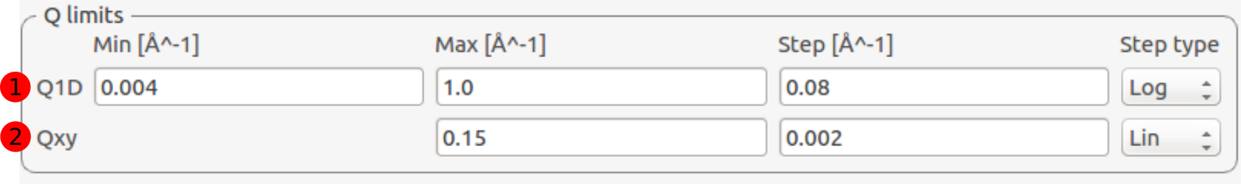
The entries here allow for the providing the binning settings during the momentum transfer conversion. In the case of a 1D reduction the user can specify standard bin information. In the case of a 2D reduction the user can only specify the maximal momentum transfer value, as well as the step size and the step type.
| 1 | 1D settings | The 1D settings will be used if the reduction dimensionality has been set to 1D. The user can specify the start, stop, step size and step type of the momentum transfer bins. |
| 2 | 2D settings | The 2D settings will be used if the reduction dimensionality has been set to 2D. The user can specify the stop value, step size and step type of the momentum transfer bins. The start value is 0. Note that the binning is same for both dimensions. |

Enabling the check-box will enable the gravity correction. In this case an additional length can be specified.
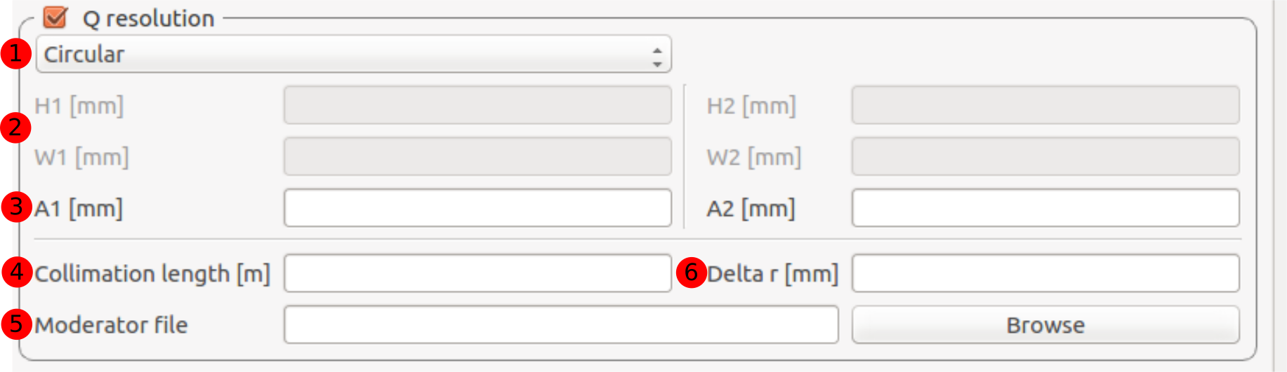
If you want to perform a momentum transfer resolution calculation then enable the check-box of this group. For detailed information please refer to TOFSANSResolutionByPixel.
| 1 | Aperture type | The aperture for the momentum transfer resolution calculation can either be Circular or Rectangular. |
| 2 | Settings for rectangular aperture | If the Rectangular aperture has been selected, then fields H1 (source height), W1 (source width), H2 (sample height) and W2 (sample width) will have to be provided. |
| 3 | Settings for circular aperture | If the Circular aperture has been selected, then fields A1 (source diameter) and A2 (sample diameter) will have to be provided. |
| 4 | Collimation length | The collimation length. |
| 5 | Moderator file | This file contains the moderator time spread as a function of wavelength. |
| 6 | Delta r | The virtual ring width on the detector. |
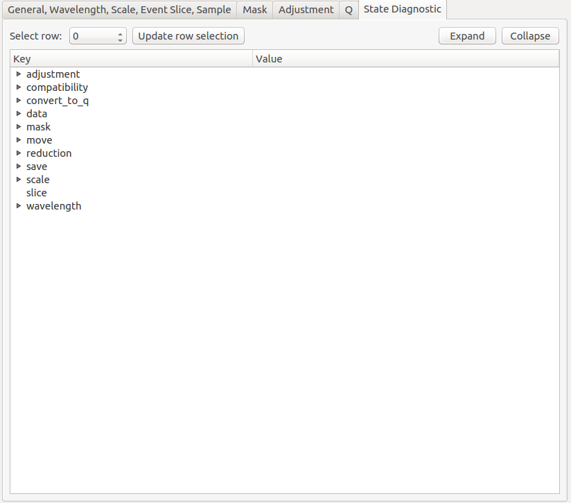
This tab only exits for diagnostic purposes and might be removed (or hidden) when the GUI has reached maturity. The interface allows instrument scientists and developers to inspect all settings in one place and check for potential inconsistencies. The settings are presented in a tree view which reflects the hierarchical nature of the SANS state implementation of the reduction back-end.
To inspect the reduction settings for a particular data set it is necessary to press the Update rows button to ensure that the most recent setting changes have been captured. Then the desired row can be selected from the drop-down menu. The result will be displayed in the tree view.
Note that the settings are logically grouped by significant stages in the reduction. On a high level these are:
| adjustment | This group has four sub-groups: calculate_transmission, normalize_to_monitor, wavelength_and_pixel_adjustment and wide_angle_correction. calculate_transmission contains information regarding the transmission calculation, e.g. the transmission monitor. normalize_to_monitor contains information regarding the monitor normalization, e.g. the incident monitor. wavelength_and_pixel_adjustment contains information required to generate the wavelength- and pixel-adjustment workspaces, e.g. the adjustment files. wide_angle_correction contains information if the wide angle correction should be used. | ||
| compatibility | This group contains information for the compatibility mode, e.g. the time-of-flight binning. | ||
| convert_to_q | This group contains information for the the momentum transfer conversion, e.g. the momentum transfer binning information. | ||
| data | This group contains information about the data which is to be reduced. | ||
| mask | This group contains information about masking, e.g. the mask files | ||
| move | This group contains information about the position of the instrument. This is for example used when a data set is being loaded. | ||
| reduction | This group contains general reduction information, e.g. the reduction dimensionality. | ||
| save | This group contains information about how the data should be saved, e.g. the file formats. | ||
| scale | This group contains information about the absolute scaling and the volume scaling of the data set. This means it contains the information for the sample geometry. | ||
| slice | This group contains information about event slicing. | ||
| wavelength | This group contains information about the wavelength conversion. | ||
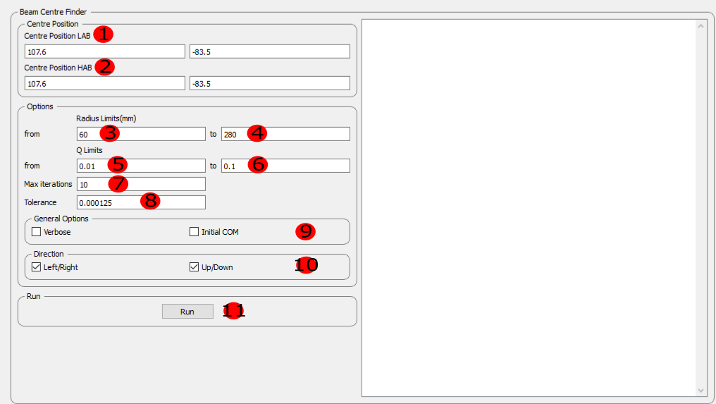
The beam centre tab allows the position of the beam centre to be set either manually by the user or by running the beam centre finder.
| 1 | Centre Position LAB | The centre position of the low angle bank. The first coordinate is horizontal and the second vertical. These boxes are populated by the user file and the values here are used by the reduction. |
| 2 | Centre Position HAB | The centre position of the high angle bank. The first coordinate is horizontal and the second vertical. These boxes are populated by the user file and the values here are used by the reduction. |
| 3 | Minimum radius limit | The minimum radius of the region used to ascertain centre position. |
| 4 | Maximum radius limit | The maximum radius of the region used to ascertain centre position. |
| 5 | Minimum Q limit | The minimum Q of the region used to ascertain centre position. |
| 6 | Maximum Q limit | The maximum Q of the region used to ascertain centre position. |
| 7 | Max iterations | The maximum number of iterations the algorithm will perform before concluding its search. |
| 8 | Tolerance | If the centre position moves by less than this in an iteration the algorithm will conclude its search. |
| 9 | General Options | The Verbose option will store the output workspaces from all iterations in memory. The Initial COM option will if checked use a centre of mass estimate as the starting point of the search rather than the user input value. |
| 10 | Left/Right | Controls whether the beam centre finder searches for the centre in the left/right and up/down directions. |
| 11 | Run | Runs the beam centre finder the boxes 1 and 2 are updated with new values upon completion. |
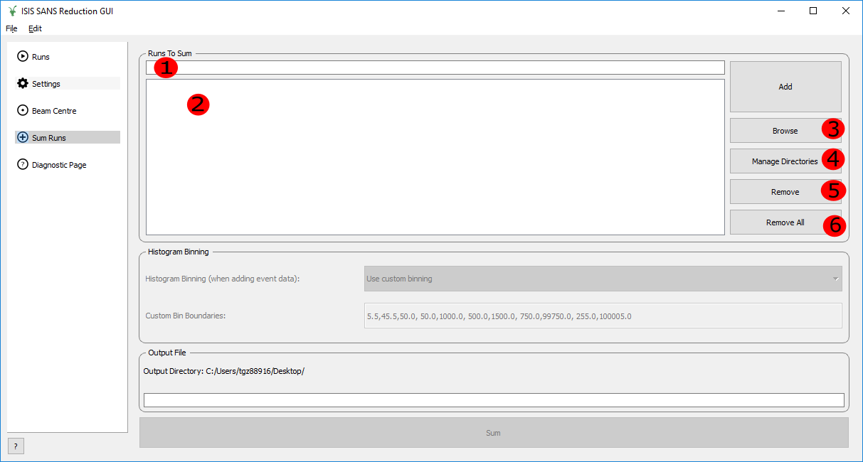
The Run Summation tab is used to perform addition of two or more run files, saving the output to a single file. The user builds a list of multiple histogram or event files (but not mixed) before pressing the sum button to produce a single output file in the mantid output directory.
| 1 | Run Query Box | This box is used to add runs to the summation table below. The user can enter one or more comma separated run numbers and press Add or the enter key to search for runs with a matching number. |
| 2 | Run Summation List | This list contains the files to be summed. |
| 3 | Browse | This button is used to select one or more nexus files to be added to the summation table. |
| 4 | Manage Directories | Opens the ‘Manage User Directories’ window allowing the user to add/remove directories from the mantid search path and to set the ‘Output Folder’ where the summation result will be saved. |
| 5 | Remove | Removes an entry from the summation table. Note, this does not delete the file itself, it just removes it from the list of files to be summed. |
| 6 | Remove All | Removes all entries from the summation table. As above, this will only remove the entries from the table, not the files themselves. |
This panel allows the user to specify the binning parameters to be applied when summing event data. There are three different ways to add files containing event data [1].
If this option is chosen a line edit field becomes available which the user can use to set the preferred binning boundaries. The format of this input is identical to the format required by the Rebin Algorithm.
A comma separated list of first bin boundary, width, last bin boundary. Optionally this can be followed by a comma and more widths and last boundary pairs. Optionally this can also be a single number, which is the bin width. In this case, the boundary of binning will be determined by minimum and maximum TOF values among all events, or previous binning boundary, in case of event Workspace, or non-event Workspace, respectively. Negative width values indicate logarithmic binning.
If this option is chosen the binning is taken from the monitors.
If this option is chosen, the output file will contain event data. The output is not an event workspace but rather a group workspace, which contains two child event workspaces, one for the added event data and one for the added monitor data.
With ‘Overlay Event Workspaces’ Disabled the event data from the files is added using the event the Plus Algorithm. Timestamps of the events and of the logs are not changed as indicated in the image below.
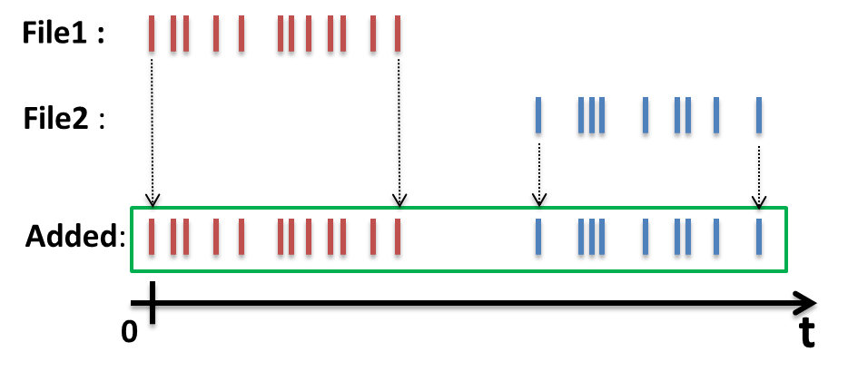
Simple addition of event data
With ‘Overlay Event Workspaces’ Enabled and no Additional Time Shifts specified, the event data of the different files is shifted on top of each other.
In the case of two workspaces the time difference between them is determined by the difference between their first entry in the proton charge log. This time difference is then applied to all timestamps of the second workspace. The second workspace is essentially laid on the first. The same principle applies if more than two workspaces are involved as this is a pairwise operation. The working principle is illustrated below:
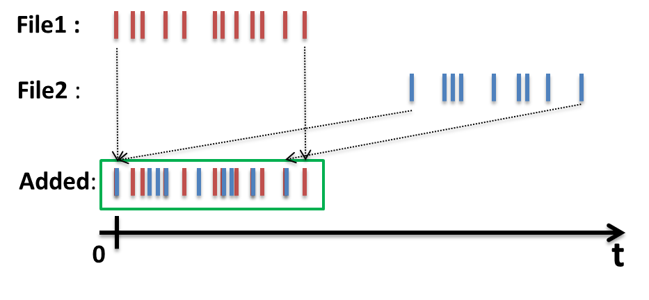
Adding two workspaces by overlaying them
Note that the underlying mechanism for time shifting is provided by the ChangeTimeZero Algorithm. Using this option will result in a change to the history of the underlying data.
With ‘Overlay Event Workspaces’ Enabled you can specify Additional Time Shifts. Additional time shifts are specified as a comma separated list of numbers where each shift is the time to shift by in seconds. The list should contain exactly N-1 entries where N is the number of runs to be summed.
Similar to the case above the workspaces are overlaid. This specified time shift is in addition to the actual overlay operation. A positive time shift will shift the second workspace into the future, whereas a negative time shift causes a shift into the past. This allows the user to fine tune the overlay mechanism. Both situations are illustrated below.
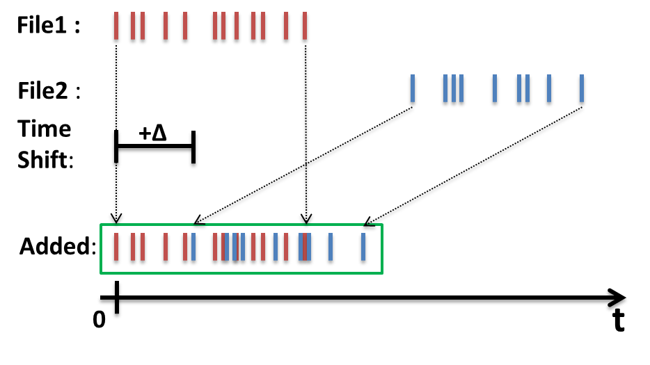
Overlaid workspaces with a positive time shift (into the future).
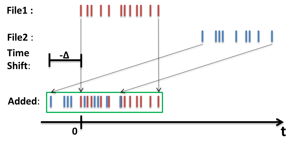
Overlaid workspaces with a negative time shift (into the past).
Just as above, using this option means that the history of the underlying data will be changed.
| [1] | These options have no effect when adding non-event data files. |
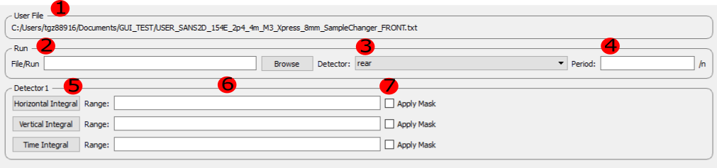
The diagnistic tab allows quick integrations to be done on a workspace.
| 1 | User File | The currently loaded user file, this is loaded on the runs tab |
| 2 | Run | The run number of file name to be considered the instrument is taken from the run tab |
| 3 | Detector | The detector to be considered |
| 4 | Period | The period to be considered if applicable if left blank will do all periods |
| 5 | Integration buttons | These three buttons start an integration on the selected workspace. The horizontal integral sums up each row, the vertical integral each column and the time integral sums across time bins. |
| 6 | Range | The range over which to do the integration. If integrating columns this is a range of rows, if summing rows a range of columns and if summing bins a range of spectra. Dashes signify a range so 1-5 for instance will integrate between rows 1 and 5 Commas signify different ranges so for example 1-5, 10-20 will intrgrate over both ranges and plot two lines Colons signify a list to integrate individually for example 5:7 is the same as typing 5,6,7 and will produce three curves. |
| 7 | Mask | If ticked the masks specified in the userfile will be applied before integrating |
If you have any questions or comments about this interface or this help page, please contact the Mantid team.
Categories: Interfaces | SANS